KISS (Karyotype Identification with Spectral Separation) Tutorial.
At Stowers we have recently developed methods for spectral karyotype analysis, sometimes known as M-FISH or SKY(TM). In the future we will put a tutorial here. For now, I will simply list the plugins needed: KISS analysis jru v1, import KISS jru v1, get KISS spectra jru v1, and KISS unmixing jru v1. The plugins for analysis of such images can be downloaded here or as a Fiji update site.
Tutorial
Acquisition
There is quite a bit of flexibility in how you collect the data. We have found we get the best results with four images per spread. The first three images are spectral images excited with 633, 561, and 488 nm excitation respectively. The spectral acquisition range is typically left constant for these. The fourth image is a DAPI image. All images should be collected with the same zoom level. You will also need to make dilute solutions of the labeled dUTP's (if you put them in hardening mounting media, you can reuse them each time) to get reference spectra. These need to be acquired with the same objectives, filters, and spectral range as the spreads.
Here is the analysis workflow:
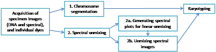
1. Segmentation
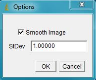
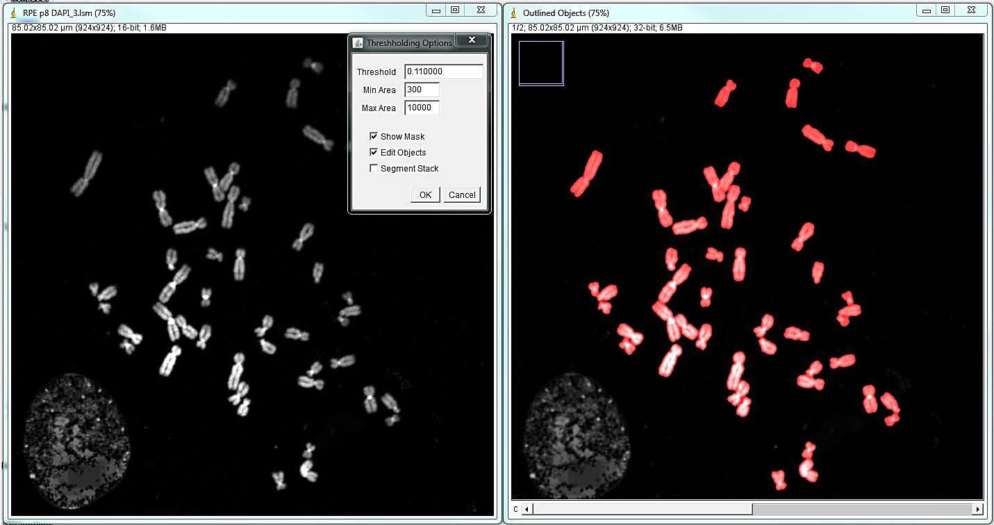
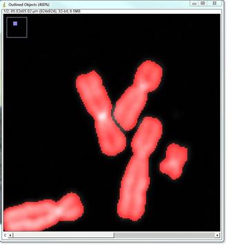
Open the DNA image; if the image has significant background - it needs to be subtracted. This can be done with the ImageJ rolling ball background subtraction: Process>Subtract Background... Select Plugins>Segmentation>outline objects jru v1. The program will prompt for the smoothing factor, which is helpful if the image is somewhat speckly. Click ok and the program will generate a new two-channel image called "Outlined Objects."
The next prompt is for thresholding options and object size (area). Select optimal parameters to segment all objects and click ok.
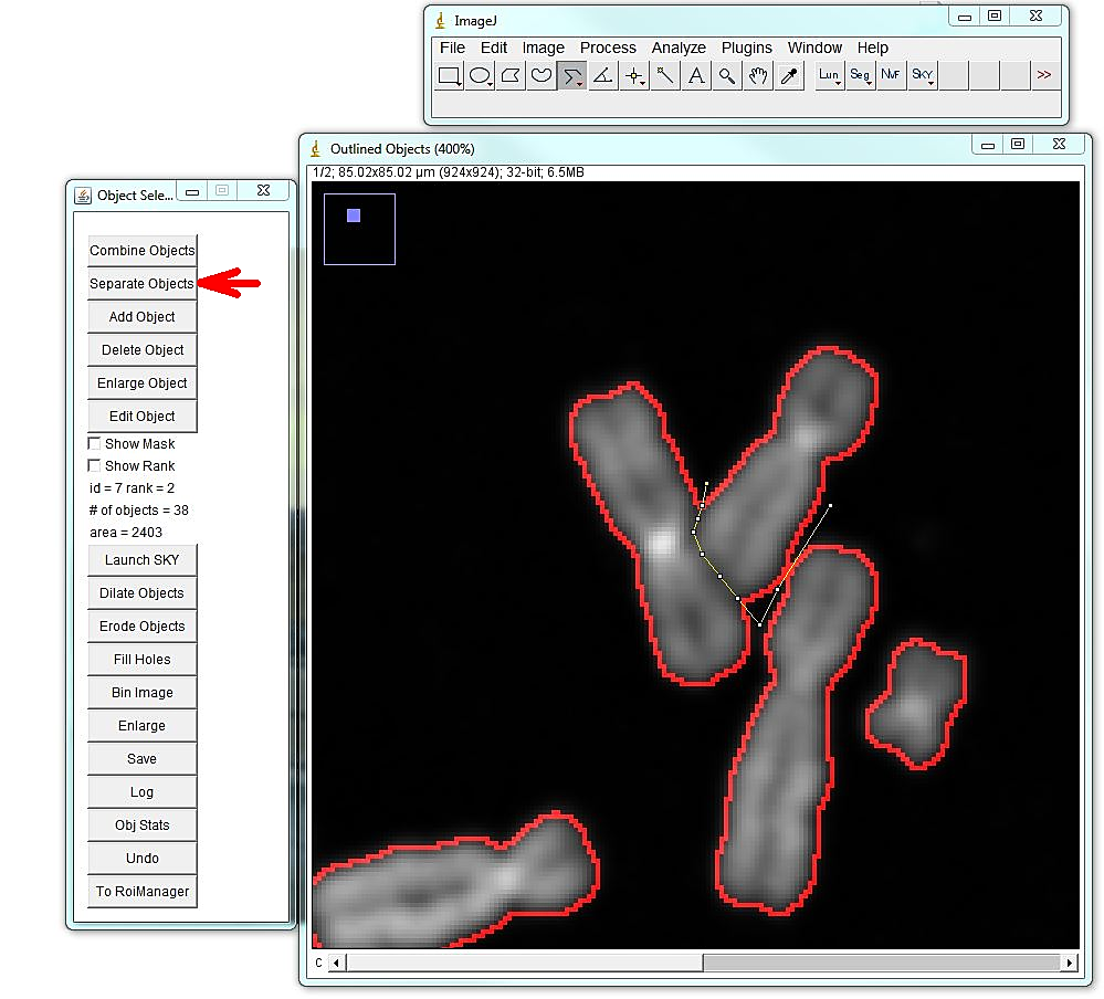
The program will open the menu that allows editing segmentation: adding, deleting, separating or merging objects, as well as saving the image and retrieving object statistics. The most common and time-consuming task is separating touching chromosomes. In the vast majority of chromosome spreads there will be chromosomes that need to be separated. To separate touching objects, use straight, segmented or freehand line tools from the ImageJ toolbar, and click "separate objects". The same tools can be used for combining objects or creating new objects. Click "show mask" before proceeding with karyotyping or saving the image. The save button on the "Object selection" tools automatically shows the masks before saving as a multi-channel tif. All objects should have masks. Note: Segmentation and identification of overlapping chromosomes are explained below.
2. Spectral Unmixing
a. Generating spectral profiles for unmixing:
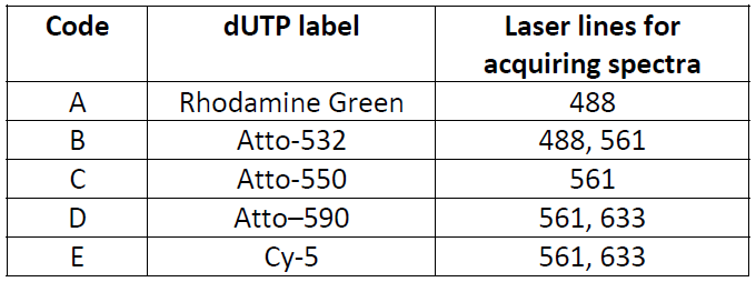
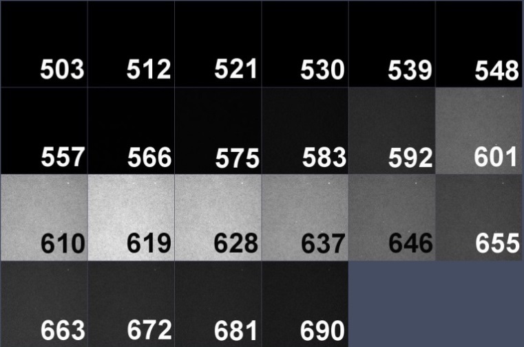
The spectral detector on the LSM 780 microscope used in this study has 22 channels, detecting emission from 503 to 690 nm. Spectral data from each chromosome spread were collected separately with three laser lines:488, 561 and 633. To perform linear unmixing, we need to know the spectral profile of each individual dye used in the probe, by creating an intensity profile (trajectory) throughout 22 spectral channels. Spectra should be acquired for each fluorescent dye with all laser lines that have capability to excite the dye (8 images total). Avoid saturation during acquisitions.
Atto-590 dUTP spectral image and spectrum with 633 laser line.
After acquiring images of each dye with indicated lasers, open all 8 images. Optionally, select spectral image regions with ROI. Run Plugins>Trajectory Tools>get KISS spectra jru v1 This generates three plot window files for three fluorescent channels containing combined normalized trajectories for that channel.
Trajectory windows must be saved as .pw2 file using the Save button in the plot window for future use for spectral unmixing.
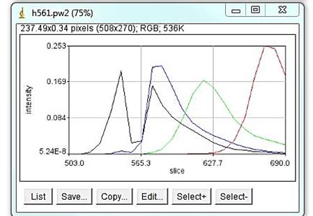
Example: combined normalized trajectories for 561 laser line including Atto 532 (black), Atto 550 (blue), Atto 590 (green) and Atto 633. The dip in Atto 532 spectra comes from a dichroic mirror.
b. Linear unmixing of chromosome spreads:
To generate the unmixed spectral image of a chromosome spread, open all three spectral images of a spread and all three .pw2 combined trajectory files:
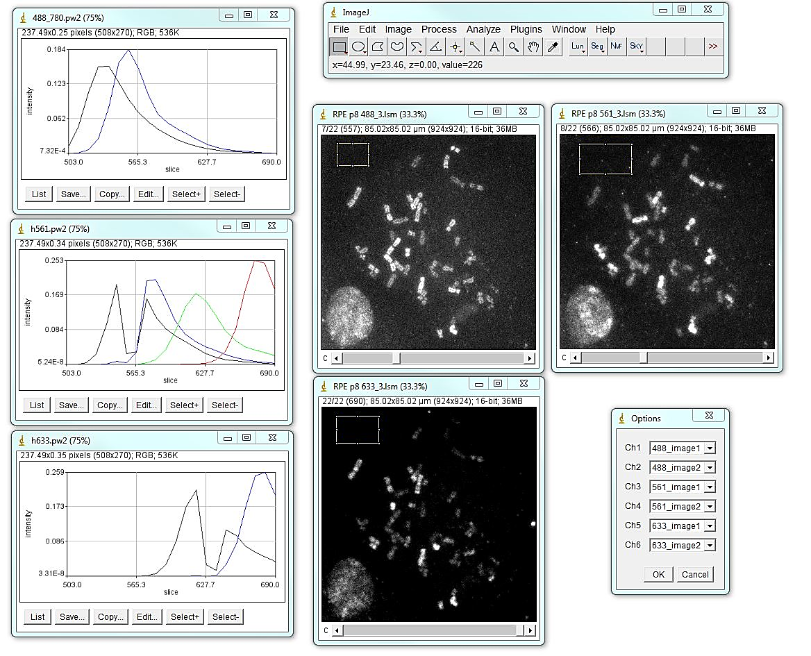
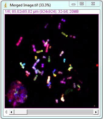
Select a background region for each image with the polygon tool. Run Plugins>Segmentation Tools>KISS unmixing jru v1. Select appropriate image files and spectral trajectory (.pw2) files and click ok. The program will prompt for the binning factor that may be useful for very large images. Note that if spectral images are binned - chromosome segmentation image should be also binned by the same factor. This can be done with the "Bin image" button on the "Object selection" tool. The unmixed image is ("Merged Image") going to have 5 channels - unmixed Rhodamine green, Atto 532, Atto 550, Atto 590, Cy5, in that order. Using ImageJ channels menu, the image can be viewed in grayscale or color mode. This image should be saved as at tiff for further analysis.
3. Karyotyping
a. Identification of chromosomes
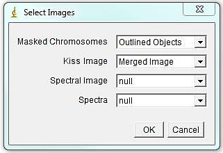
To start karyotyping the chromosome spread, open two images generated in previous steps: 1-segmentation file "Outlined Objects", and 2-unmixed stack "Merged Image". If the merged image was binned in the KISS unmixing step and the DAPI image was not, bin the segmented DAPI image by the same factor using "Bin image" button in the "Object selection" menu.
Run Plugins>Segmentation Tools>KISS analysis jru v1 and choose appropriate image names for masked chromosome image and unmixed KISS image; select "null" for "Spectral Image" and "null" for "Spectra".
*** Advanced Note: If the spectral data was collected in one file with all three laser lines simultaneously, you can select the multi-laser file in the "Spectral Image" window, and the assembled spectral .pw2 file in "Spectra" window.
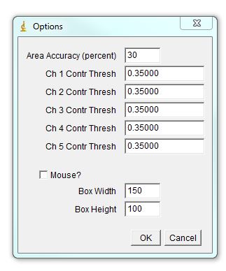
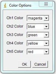
The program will bring out a prompt window for several parameters that contribute to assigning chromosomal identity: 1. Area accuracy - this determines how much the size of a chromosome is taken into account when assigned identity. Lower number means more stringency, 100 eliminates size consideration. 2. Channel Contribution threshold - this is the threshold for a chromosome to be considered "positive" for a specific label. If one if your labels has particularly high background, select a higher value here. For a weak label, a lower value may help. 3. Mouse - Check if analyzing mouse karyotype. The program defaults to human karyotype unless this box is checked. Box width and height determine dimensions of karyotyping window. The karyotype below is 120x120. You can always reload the karyotype and increase this parameter later if necessary. Next select the desired color for each channel or leave defaults. Click ok.
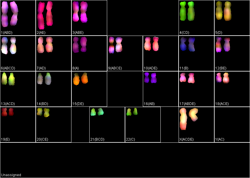
The program opens a window called "Karyotype" with automatically assigned chromosomes using parameters specified previously. Chromosomes are colored according to the normalized dye contribution in each pixel multiplied by the selected color for that dye. In addition, program opens the "KISS image" and "KISS analysis" windows. These windows are interactive. Selecting an object in "Karyotype" window using by clicking highlights the selected object in the Karyotype window, as well as in "Outlined Objects" and "KISS" image. This allows visual and spectral inspection of a chromosome in detail. "KISS analysis" window shows relative spectral composition of a selected object and corresponding assignment.
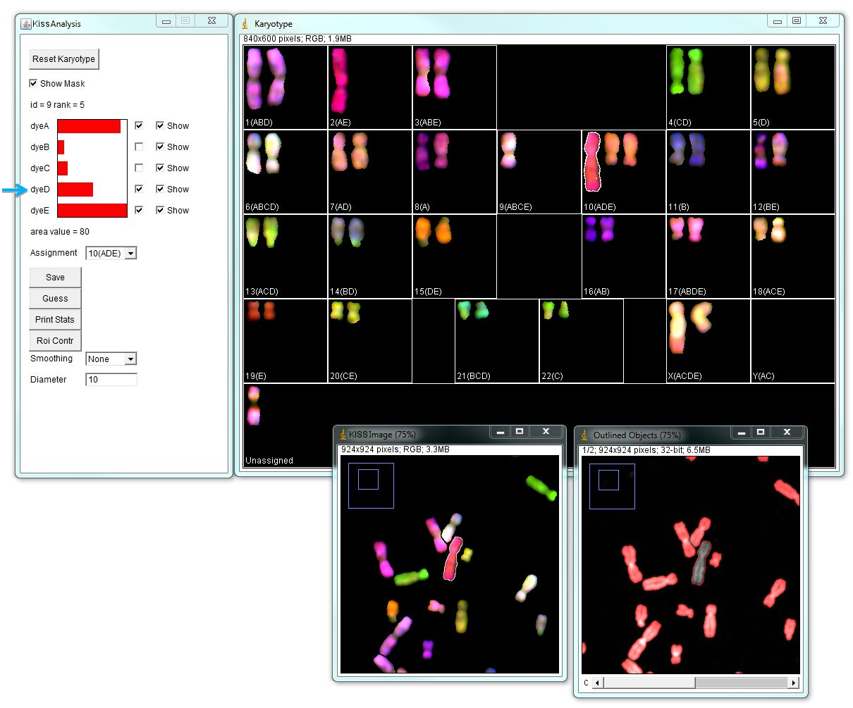
Typically automatic chromosome assignment is not perfect and needs to be corrected manually. There can be chromosomes that are assigned identities incorrectly or remain unassigned. In the example below, there is a large metacentric chromosome assigned as Chr.10 (ADE), which given its color and morphology is likely wrong, because chromosome 10 is medium sub-metacentric. The "KISS analysis" window shows major contributions from channels A and E, and some contribution from channel D that passes the 0.35000 threshold. However, given this chromosome’s morphology and spectral composition most likely this is chromosome 2 (AE). Unchecking "dye D" will assign this chromosome as chr.2.
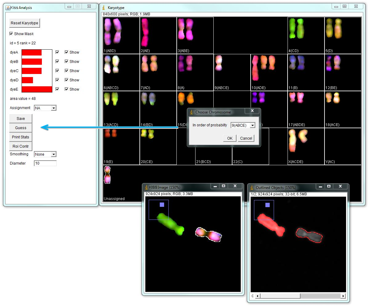
Using the "Guess" button in the "KISS Analysis" window arranges chromosome identities in the order of probability for the selected object. In the example below, the "unassigned" chromosome is selected and its spectral contributions are shown in the "KISS Analysis" window. Again, channel D passes 0.35000 threshold, but its contribution is lower than other channels. "Guess" option indicates that this chromosome is most likely the chromosome 9. Click OK to move this chromosome in selected position.
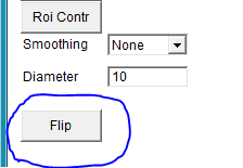
Use the "Flip" button to rotate up-side-down oriented chromosomes P-arms up (180 degrees), if desired.
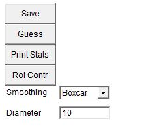
b. Smoothing the KISS Images
The chromosome painting probe derived from single-sorted chromosomes does not give a labelling with uniform intensities - the intensity of a signal can vary throughout the length of chromosome arms. Therefore, the KISS image may appear non-uniform and this may visually look similar to translocations. Smoothing the chromosomes allows for easier chromosome identification. Such smoothing can be undone later for fine translocation assessment if desired. To smooth the image, the KISS analysis window has two options: one option is to replace each chromosome with its average ("Show_Avg"). This flattens the color but also masks tranlocations. The "boxcar" option is more useful because it limits blending of one region of the chromosome with another. The diameter box beneath the smoothing selection gives the diameter for the boxcar smoothing. The default value is 10. Larger diameters take longer to update in the karyotyping window. Here is an example with boxcar smoothing diameter of 10.
c. Dealing with overlapping chromosomes:
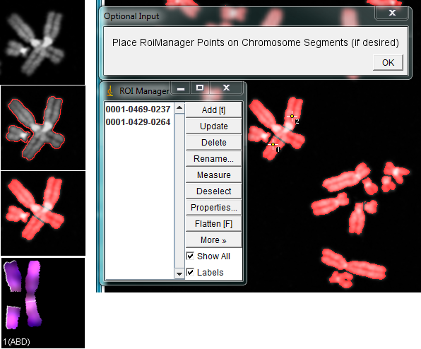
1. Segmentation: to segment overlapping chromosomes, first they are segmented as one object, and then separated at the borders of overlaps. Sometimes, it is better to exclude region of the overlap altogether; other times one of the overlapping chromosomes may be left intact, as in the example above. However, the spectrum of the overlapping region may affect chromosome identification, if the spectrum of the spectrum of underlying chromosome pollutes the spectrum of the intact chromosome.
2. Karyotyping: when running KISS analysis jru v1 plugin, it will prompt to add points to the ROI manager identifying pieces of the same chromosome. Select the point tool from the ImageJ main menu, click on the first piece and press "T", then click on the second piece and press "T" again and click Ok. This will link the two pieces of the chromosome together. Do this for all pieces of overlapping chromosomes and click Ok.
In the karyotyping window, chromosome pieces will remain linked, maintaining a gap the size and shape of the excluded overlapping region.
d. Discerning translocations:
When a translocation is suspected, it is of interest to determine the spectral composition of a certain region of a chromosome. Select the region of interest with one of the selection tools in ImageJ main menu and click "Roi Contr" in the KISS analysis window. It brings out a window with spectral contributions in the selected region of interest. In the example below, the spectral composition of the entire X derivative is ACDE (chr. X), while the selected region is ADE (chr. 10).
"Show" checkboxes the the KISS analysis window allow toggling views of specific dye channels in the image for examining color patterns. Unchecking the "Show" box excludes that channel from the color palette. The karyotype of the RPE1 cell line is known to have an additional piece of chromosome 10 at the end of the Q-arm of one of the X chromosomes. In the example below, turning off channels A, B, and D highlights the derivative X chromosome.
When a tranlocation is presumed, it is highly recommended to go back to the unmixed "Merged Image" and examine the chromosome of interest thoroughly in all channels.
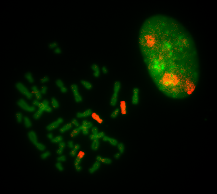
Translocations should be subsequently confirmed with single chromosome-specific probes or by sequencing methods. Here, a spread from the RPE1 cell line is labeled with a single probe specific for chr. 10.
Note: Satellite DNA (ribosomal DNA repeats) on short arms of human acrocentric chromosomes (13-15, 21, 22) stains differently than the rest of the chromosome, and should not be mistaken for translocations.
In a mouse, all chromosomes are acrocentric and their short arms may also be stained differently than the rest of the chromosome.
5. Saving and opening karyotypes (.kiss files):
You may want to save karyotypes for further viewing or work, or to change the size of the karyotype boxes. To save the karyotype, click the save button on the "Kiss Analysis" window. The files shouls be saved with the ".kiss" extension. You can load these files with the Plugins>File Tools>import KISS jru v1 plugin. Drag and drop as well as the File>Open command should also work but can have issues. Note that window dimensions and flipping are not saved.
In the dialog that appears after opening, do not change area accuracy and contribution thresholds since previously assigned chromosome identities are stored in the .kiss file. Check the "Mouse?" box for mouse karyotypes. Check "Output Unmixed" to open the unmixed merged image. If you make further changes to the karyotype, you need to resave to preserve them.

6. Customizing the code:
You may run into a scenario where you would like to change the probe contribution code because of a particular issue identifying a chromosome. To do this, use the Plugins>Segmentation Tools>edit KISS codes jru v1 plugin. You can pick one of the default code sets to start. The code will get saved to your profile on the computer you are currently using. On windows computers, this is in c:\Users\username\ImageJ_Defaults\edit KISS codes jru v1.jrn. The file is a simple text file. You can select the custom code from either the KISS analysis jru v1 plugin or the import KISS jru v1. Note that the code doesn't get saved with the karyotype. You need to reimport it every time you perform an analysis or reload a previous analysis.