Particle Tracking Plugins ("track max not mask")
Here I will describe a set of particle tracking plugins (track max not mask jru v2 and track max not mask 3D jru v1) that we also utilize for segmentation of crowded environments. Under these conditions the plugins outperform traditional segmentation algorithms because they rely on uniformity of size among structures--something that is difficult to implement in purely threshold based segmentations.
Update: I have recently implemented fast versions of the above plugins. They work in much the same way, but perform the object identification (the track max not mask portion) in a tiled fashion, combining the points from the tiles to create the whole data set after the fact. This speeds up analysis significantly but may result in slightly different object positioning at the tile boundaries especially from dense images. These plugins are called track max not mask fast jru v1 and track max not mask 3D fast jru v1.
Algorithm
These plugins are not novel in the algorithmical sense--they are based on a very simple premise. In that respect, they are certainly not the most computationally efficient way to track maxima in an image, nor do they strictly find only true maxima in an image. The "Find Maxima" tool built into ImageJ outperforms this algorithm in terms of computational performance and the restriction to true maxima. Nevertheless, I prefer this implementation when possible because it outperforms more sophisticated implementations by finding dim neighboring blobs when they do not represent true maxima. Note that the 3D implementation is identical to the 2D implementation but in three dimensions.
Firstly, the algorithm finds the maximum intensity pixel in the entire image. All pixels within a specified radius around that maximum are deleted ("masked"). Then the maximum value is found again and masked until there are no pixels above the threshold value. The threshold is determined based on the fraction of the maximum intensity in the image.
After maxima are found in this way, they are tracked in a relatively simple fashion. For each point, the closest neighboring point in the subsequent frame is identified as the same object in the next frame as long as it is below the distance (Link Range) cutoff. If a particle has disappeared in the next frame, it should reappear before Max Link Delay number of frames or it will be considered a new particle.
Usage
Prior to running these plugins, the user should duplicate out the desired image channel and appropriately subtract the background (using roi average subtract jru v1 or Process>Subtract Background). In addition, if the objects to be tracked have significant internal heterogeneity, it is a good idea to blur them (possibly in 3D) with Process>Filters>Gaussian Blur to reduce them as much as possible to single maxima.
The plugins are interactive. This means that for a small image, you can adjust the parameters to get the best maximum identification in an interactive way. The negative impact of this is that it is very crash prone for large scale images. I would recommend recording a macro with a small scale image and then running that macro on larger scale images to avoid crashes.
A reasonable demonstration data set for the plugin is the mitosis sample video built into ImageJ (File>Open Samples>Mitosis). The red channel contains multiple blobs that move in time. These blobs are relatively sparse, so we will track them in 2D on the max projection. To begin with, duplicate the first 25 frames of the red channel and convert it to grayscale with Image>Lookup Tables>Grays. Then we will use the ImageJ Subtract Background utility with a rolling ball radius of 10 pixels. Then to denoise the image somewhat, we will use the Gaussian Blur utility to blur with a radius (standard deviation) of 1 pixel.
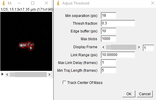
Next, run the track max not mask jru v2 plugin. We will threshold relative to the maximum intensity statistic. Tracking parameters that worked well for me were a min separation of 18 pixels, a threshold fraction of 0.3, and all other parameters at their default including track center of mass. I rarely use this option for crowded environments even though it may track more accurately for less crowded environments. You can use the display frame slider to visualize the tracking as it occurs. If the program is jumping too easily between particles, try reducing the link range. The min traj length parameter is simply a filter to eliminate noise and ephemeral particles.
After tracking is complete, a plot will appear with the trajectories on it in addition to a large table containing position and intensity information. You can save the plot as PlotWindow file using the "Save" button on the plot window. This can be reloaded into ImageJ for further analysis.
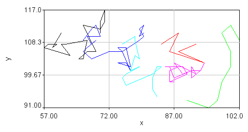
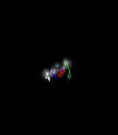
Visualization of the trajectories is perhaps best accomplished using tools outside of ImageJ. However, for quick checks of the tracking performance, one can use traj 2 roi jru v1. Using the overlay option shows all of the trajectories as a static overlay on the movie. Choosing the trails option along with trails persist gives a movie of the trails. Those can be overlayed on top of the original movie with the plugin overlay image jru v1.
Alternative Application: Nuclear Segmentation
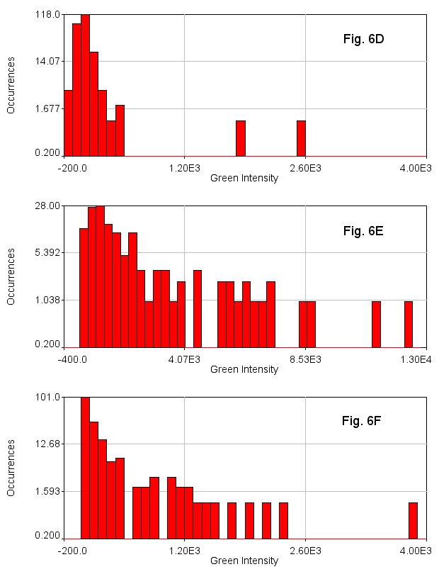
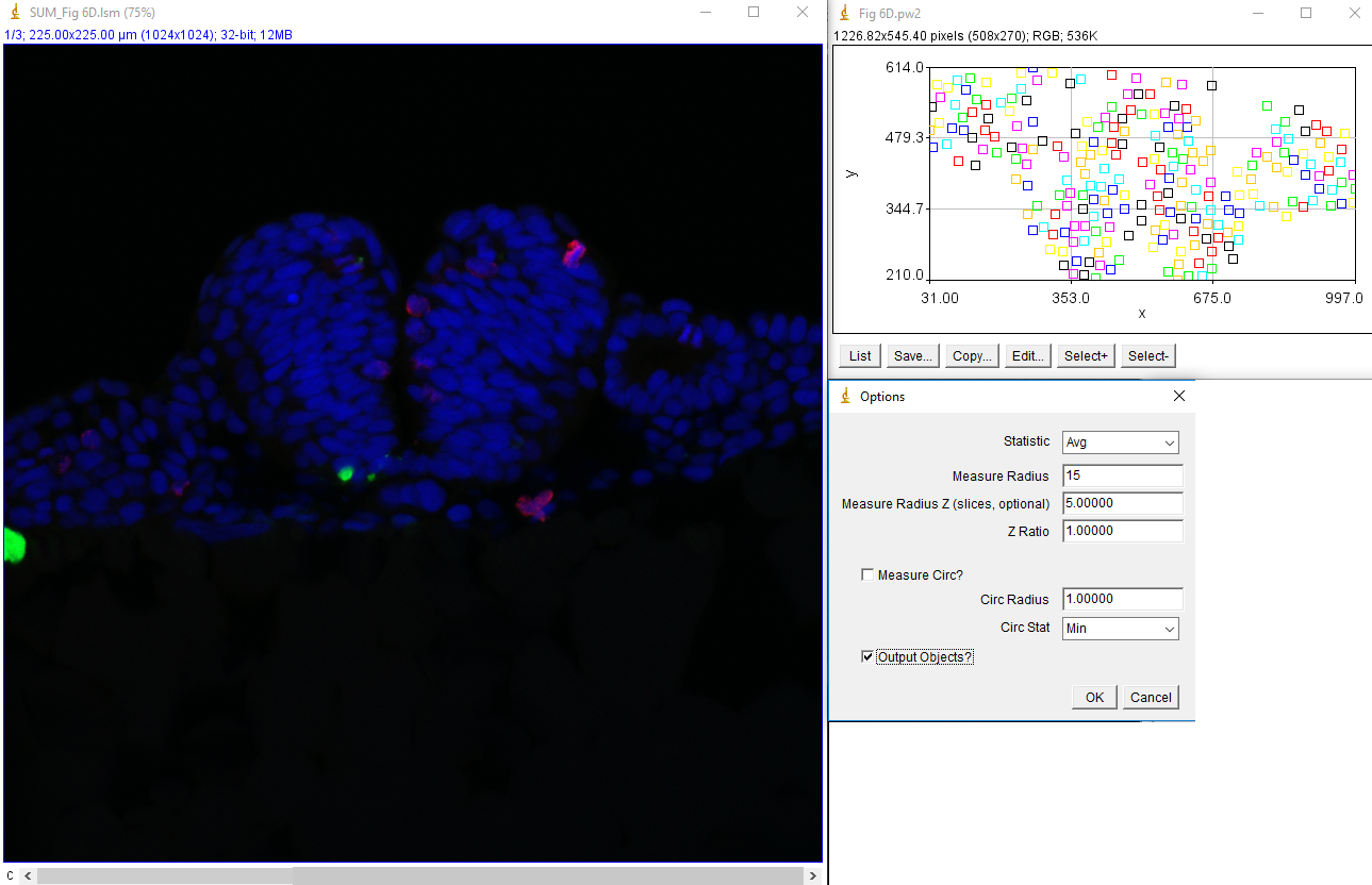
In addition to being useful for particle tracking, these plugins are also useful for quasi-segmentation, especially for crowded circular objects. As you will see, the segmentation is not perfect--some objects are split into two, especially if they are elongated. Nevertheless, the density of objects is representative of the density of nuclei in the image in such a way as to provide an unbiased assessment of the distribution of nuclear intensities. As an example, we will use data from Watt et. al., 2016, PLoS Genet., Figure 6D-F. This data is publicly available here. For simplicity, we will sum project (Image>Stacks>Z Project) from slice 5 to slice 10 which approximately covers a single nuclear depth. Next we duplicate the DAPI channel (channel 1) for tracking. Next, we Gaussian blur with a radius of 7 and subtract a rolling ball background with a radius of 100 pixels. Then we run track max not mask jru v2 with a min separation of 50 pixels, and a thresh fraction of 0.3. Note that we need to set our min traj length to 0 since we are not tracking objects through time here.
After running the plugin we get the expected table and trajectory plot. The table is useless since it contains only DAPI intensities which we are not interested in. The trajectories plot appears blank because all of our trajectories are a single frame in length. They can be made visible with the plugin "set 3D shapes jru v1".
Note also that the plot of nuclear positions will appear inverted because the 0 y coordinate is at the top of the image but at the bottom of the plot. You can obtain a plot that looks more like your image but clicking the Edit... button. Then set the x min and x max values to 0 and 1024 and the y min and y max values to 1024 and 0. Finally, you can make the plot appear square by setting the Mag Ratio parameter to 1.
Now that tracking is complete, we want to measure the intensity of the green and red channels within these nuclei in the sum projected image. This is done with measure trajectories jru v1. First, subtract the background of the sum projected image by selecting a region outside the signal areas and running roi average subtract jru v1. Set the measure radius to 15 to match our cell size approximately. This value can be reduced to measure only in the center of the nucleus or enlarged to measure the border surrounding the nucleus. I like to select the output objects option to see what regions exactly are getting measured. These will be indexed by a unique intensity in the output image. If you only want to measure the border of your nuclei, use the measure circ option with the selected radius (thickness) and statistic. The resulting statistics will be output in a table with channels labeled by number.
While our example images had different levels of green intensity (either due to staining differences or microscope acquisition parameters), the intensity histograms make it quite clear that 6E has many more green cells than 6D and 6F has an intermediate number of green cells.