Single Particle Averaging Super-Resolution Tutorial
Introduction
Single particle averaging super-resolution microscopy is a method to improve dramatically the signal/noise ratio in such images (Reference 1). The method is fairly simple for highly symmetrical structures with recognizable features. First the images are realigned to a common axis with a common resolution. After realignment, the structures are combined into a pseudo time series with each "frame" being a different realigned image. Finally, the images are averaged together. Note that these tools assume a homogeneous set of structures. Structural heterogeneity will be averaged out. Here I will describe how to use the tools for 3D realignment and averaging of spindle pole bodies (Reference 1) and synaptonemal complex structures (Reference 2). The plugins can be downloaded here or as a Fiji update site.
2D synaptonemal complex alignment
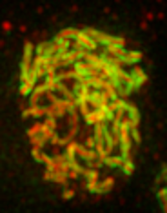
Two dimensional SPA-SIM is perhaps the simplest form of single particle averaging in the same way that linear fiber Cryo-EM with a highly repetitive fiber is simpler than traditional single-particle EM. This is because alignment is only necessary along one axis. We will perform SPA-SIM to obtain the average structure of C(3)G and corolla in the Drosophila synaptonemal complex. A sample image can be downloaded here. Looking at the maximum projection image below it is clear that the fibers are composed of two parallel tracks in the C(3)G channel (channel 2) and a single track in the corolla channel (channel 1). Nevertheless, in many places the tracks are noisy and it is difficult to assess the track spacing and the exact positioning of the corolla track between the C(3)G tracks.
It is relatively straightforward to find tracks travelling parallel to the plane of focus when looking at each 2D slice. We will draw lines perpendicular to the fiber tracks as shown below:
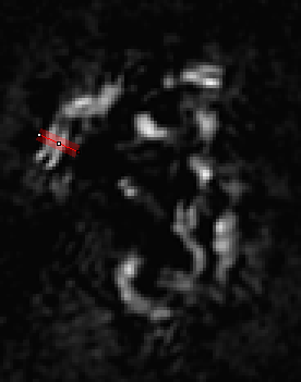
In ImageJ, the thickness of lines is changed by double clicking the line tool. The correct value to choose depends on the application, but I would suggest choosing the thickest value that still gives a straight track selection. Obviously if the track is curving within the thickness of the selection, our reconstructions will appear blurred due to curving rather than actual structural variation. I used a thickness of 4 for this application. I recommend adding the selections to the RoiManager (Press "t") for later reference. I like to save the final roi list by deselecting all roi's and running More>Save on the roi manager. That allows me to go back and look at each roi later if desired. The next step is to create averaged one dimensional roi profiles. For this, run Plugins>Stowers>Jay_Unruh>polyline kymograph jru v1. The "Profile Width" value will initialize to your line roi width. Select "Single Frame Profile" and "All Channels (for single frame)" and click ok to the the line profile.
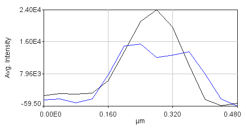
Note that the colors are a bit different for plots than for the images. If you click "Select +" on the plot multiple times, you can cycle through the channels. Black is channel 1 and blue is channel 2. Once you have done this for all of the desired lines, combine them together with Plugins>Stowers>Jay_Unruh>combine all trajectories jru v1. Make sure you don't have any other plot windows open. Start by combining the 2nd channel. Note that if you try to combine all trajectories again, the combined 2nd channel will be added to the list. So save the plot window using the "Save..." button on the plot and close it before combining channel 1. You can then reopen it with File>Open or with Plugins>Stowers>Jay_Unruh>Trajectory Tools>import plot jru v1. The rest of the procedure basically consists of aligning these profiles to their centers. In order to find the centers accurately, we need to fit the Channel 2 profiles to double gaussian functions. This is done by selecting each profile with the "Select +" button and running Plugins>Stowers>Jay_Unruh>Trajectory Tools>fit traj double gaus jru v1. The results are appended to the "Double Gauss Fits" table which can be copied to a spreadsheet for further processing. I used a standard deviation guess value of 0.05 microns and min and max standard deviation values of 0.01 and 0.075 microns respectively. Note that some profiles simply will not be fit and therefore need to be removed from the plot window by selecting them and then pressing the "Edit" button on the plot and selecting "Delete Selected." Don't forget to delete that series from both channels profiles. In addition you will need to remove their values from the table. This can be done after copying to a spreadsheet program. It is important to note at this point that the profile fits are very informative apart from the SPA-SIM process itself. From the 8 profiles I generated for this example, I find that the average peak standard deviation is 0.046 microns. The width of a Gaussian function is 2.35 times the standard deviation, giving a width of 0.107 microns, very close to the reported resolution of the SIM microscope. The average distance between peaks is 0.137 microns--very close to the reported value for C(3)G.
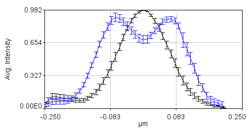
The next step is to align all of our profiles to the center. This is done by running Plugins>Stowers>Jay_Unruh>Trajectory Tools>set multi plot offsets jru v1. The input is a large text window, so just copy the xc values from your spreadsheet (one single column, one after another) into that window. This will center all of the profiles at 0. Remember to do this for channel 2 as well. Note that all this plugin does is to subtract a value from the x axis. If we average the profiles together at this point, the data points will not line up. To remedy this, run Plugins>Stowers>Jay_Unruh>Trajectory Tools>resample plot jru v1. I typically choose an X Increment value of 0.01 microns and use the default start and end values. Optionally, you can normalize the profiles so that they are similar heights with Plugins>Stowers>Jay_Unruh>normalize trajectories jru v1. If you don't do this, the errors will reflect intensity differences rather than profile shape differences. The next step is to calculate the average profiles with Plugins>Stowers>Jay_Unruh>Trajectory Tools>average trajectories jru v1. Here is the result of our data set:
Note that in order to copy the values from this plot, simply click the copy button on the plot and paste to a spreadsheet program. To copy the errors, run Plugins>Stowers>Jay_Unruh>Trajectory Tools>copy errors jru v1.
3D spindle pole body alignment
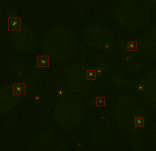
Note that this protocol should work for any structures which are radially symmetric and have two relatively circular spots to use as fiducial markers. For our example, we will use mTurquoise2-Spc42-YFP at the yeast spindle pole body as published in reference 1. A sample image can be downloaded here. These cells are arrested in alpha factor and should have duplicated Spc42 satellite spots. First we need to duplicate small subregions cropped around those two spots. This is done most easily on a sum projected image. This is created by running Image>Stacks>Z Project. Select the entire range and the sum statistic. Then select the double spots as in the image below.
You will probably need to play with the contrast to make it easy to find the appropriate structures. I use the roi manager to store all of the roi's and transfer them from the sum projection to the full 3D image.
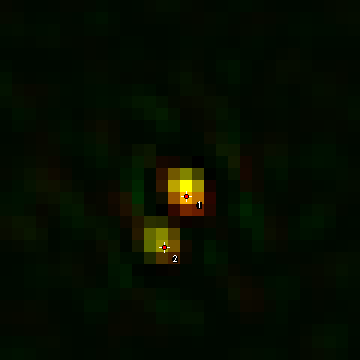
Next, I duplicate all of the roi's from the roi manager and the 3D image using Image>Duplicate. As you duplicate the roi's, double check that the spots don't have their maximum intensity in the first or last slices. If they do, delete the corresponding roi in the roi manager as well as the duplicated image. I like to save the final curated roi list by deselecting all roi's and running More>Save on the roi manager. That allows me to go back and look at each roi later if desired. The next step is to fit the mTurquoise2 spots in each duplicated image to 3D Gaussian functions and realign both channels along the fitted axis. Once all sub-images are duplicated, empty the roi manager and select two spots using the spot selection tool in channel 1 on one of the duplicated images. Always start with the brighter spot first. This spot corresponds to the mother spindle pole body. Use single spots and the roi manager, not the multispot tool. Here is an example:
Once the spots are selected for each image, I typically save each duplicated image, again in case of future analysis or investigation. If you have the show all option selected in the roi manager, you can reload the images and get the roi's from the overlay later. Make sure the channel slider is on the channel you want to fit. In this case it is channel 1 (the yfp channel). Fit the rois using fit Plugins>Stowers>Jay_Unruh>Image_Tools>fit 3D multi gaussian jru v1. Z Ratio is the ratio of the z resolution to the xy resolution. For our images this is 125 nm/40 nm = 3.125. The initialized StDev guess values should work well. Also, leave the Calibrate and Show 3D Plot options checked. The plugin will output five windows. The "Avg Projections" 3D plot shows the xy average projections and fit surfaces. The "fit" image shows the same thing but in an image representation. The "Z Profiles" plot shows the Z intensity profile of the data and fit for each spot. This is another opportunity to make sure your spots are not at the upper or lower slices. The "MultiGaus Plot" 3D plot is the only window we will use going forward, so you can close the others after checking them. Note that there is also a table of fit values which you can retain if desired. Future fits will add to this table if you leave it open.
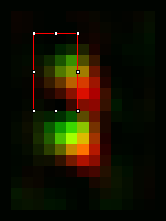
To realign the original image, run Plugins>Stowers>Jay_Unruh>Segmentation Tools>thick 3D polyline profile jru v1. Select the "MultiGaus Plot" for the 3D profile and the duplicated 3D image. Here I use a thickness of 15 and an end extension of 1.5 (continues the profile 150% beyond the end of both spots). Also select the "Straighten" option to get the realigned image rather than the intensity profile. I typically select the "Single Slice" option if the interesting information is confined to the inter-spot axis. Once the realignment is complete, save the realigned image. I typically save it with "_realigned" appended to the file name. This allows for batch import and averaging later. Here is a realigned image example:

Once a significant number of images are saved (we typically use >30 images but more or less may be necessary depending on the quality and homogeneity of the images), it's time to average them. Start by closing all open images in ImageJ. Then open all of the realigned images you saved earlier. I use the Plugins>Stowers>Jay_Unruh>File Tools>batch file open jru v1 to open all of the desired images. Here is where having a common substring (like "_realigned") in the image name comes in handy. Then merge the opened images into a time series with Plugins>Stowers>Jay_Unruh>Image Tools>merge all stacks jru v1. This plugin centers each image as it merges them together, padding the edges with zeros. Note that our current methodology doesn't distinguish between spindle pole body objects flipped to the left or the right of the realignment axis. In ref we chose to flip them all to the right side. This is accomplished with Plugins>Stowers>Jay_Unruh>Misc Tools>flip roi mirror right jru v1. Firstly, make sure the secondary channel is selected with the channel slider. Next draw an roi on the left hand side encompassing the left side of the spindle pole signal as follows:
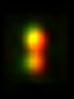
The plugin will measure the intensity of this roi along with its mirror to the right. If the mirror is brighter, the image is flipped. If not, it is retained. Finally average the images with Plugins>Stowers>Jay_Unruh>Image Tools>bin image jru v1, selecting temporal binning. Here is the result averaged and then scaled a factor of 8 with bilinear interpolation:
References
1. Burns S, Avena JS, Unruh JR, Yu Z, Smith SE, Slaughter BD, Winey M, Jaspersen SL. Structured illumination with particle averaging reveals novel roles for yeast centrosome components during duplication. eLife. 2015;4. Pubmed
2. Collins KA, Unruh JR, Slaughter BD, Yu Z, Lake CM, Nielsen RJ, Box KS, Miller DE, Blumenstiel JP, Perera AG, Malanowski KE, Hawley RS. Corolla is a novel protein that contributes to the architecture of the synaptonemal complex of Drosophila. Genetics. 2014;198:219-228. Pubmed