Fluorescence Correlation Spectroscopy, Brightness Analysis, and Photon Counting Histograms
Fluorescence Fluctuations
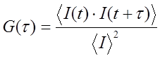
The basis for FCS and its related techniques is brownian diffusion and the statistics of molecular occupancy. The focal volume of a confocal fluorescence microscope is less than 1 femtoliter (we estimate ~0.1 fL for a confocal microscope with a small pinhole). As a result, a 100 nM solution of fluorescent molecules will have on average 6 molecules in the microscope focal volume at a time. Clearly, molecular diffusion will cause molecules to diffuse in and out of the microscope focal volume. This is accompanied by fluctuations in the fluorescence intensity measured by the microscope. Given the fast time scales involved and the low fluorescence from most fluorophores of interest, the appearance of the time trace simply appears as a noisy signal. To extract information about the fluctuations we need to calculate a temporal autocorrelation function. This calculation is conceptually fairly simple: the time trace is copied and shifted by one time point and the correlation coefficient is calculated. Then the copied trace is shifted by two time points and correlated again. This is repeated for all possible time shifts. For small shifts, the correlation will be high because the traces are very similar. As the shifts get bigger the fluctuations will be widely separated from one another and the correlation will go to zero. Here is the correlation calculation in mathematical terms:
Here is a simulated trace and its temporal correlation:
References:
Elson, E. L. and D. Magde (1974). "Fluorescence correlation spectroscopy. I. Conceptual basis and theory." Biopolymers 13(1): 1-27.
Analyzing the Correlation Function
There are typically two basic pieces of information that can be gleaned from the correlation function: the average time it takes for a molecule to move through the focal volume, and the number of particles in the focal volume. For simple diffusion in two and three dimensions, this relationship is given as follows:

Here τd is the average time required for a molecule to traverse the radial dimension of the focal volume, γ is a shape factor for the focal volume, N is the average number of molecules in the focus, and r is the ratio between the axial and radial dimensions of the focal volume. Often the ratio γ/N is referred to as G(0) because it describes the amplitude of the correlation function at zero time lag. The diffusion time is directly related to the radial dimension of the focal volume as follows:

Here ω0 is referred to as the "beam waist" of the focal volume. It is related to the full width half maximum (FWHM) as follows:
This analysis assumes a 3D Gaussian microsope focus:
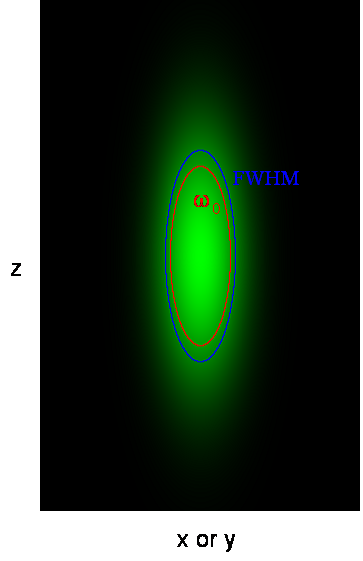
This is a good approximation only for a small pinhole. Mathematically this focal shape is given as follows:
References:
Thompson, N. L. (1991). Fluorescence Correlation Spectroscopy. Topics in Fluorescence Spectroscopy. J. R. Lakowicz. New York, Plenum Press. 1: 337-378.
Calculating Concentration
Given the simple relationship between the correlation function amplitude and the average number of particles, it seems straightforward to immediately calculate the particle concentration. All that is missing is the volume of the focus, right? Unfortunately, the answer is not that simple. Theoretically, the volume of the focus is given by the integral of the 3D Gaussian laser focus as follows:

Here we already run into problems. In principle, the z0 parameter in the above equation can be determined from the axial/radial ratio defined above, but in practice, this measurement is only weakly sensitive to the actual axial dimension of the focus. In fact, recent papers (Hess and Webb) recommend fixing this parameter to a value of 5 in the analysis. The rational for this lies in the poor z resolution inherent to optical measurement techniques. During the fluctuation measurement, the changes in intensity as the molecule moves radially are much greater than those accompanying axial motion. As a result, one can essentially omit information about the third dimension from FCS analysis and still get reasonable results.
Further complications are given by the nature of the correlation amplitude measurement itself. While FCS is uniquely sensitive to the fluctuations of single molecules, its amplitude is notoriously dependent on background fluorescence intensity. In fact, every confocal measurement has significant amounts of out of focus light that contaminate every measurement. Since this light spreads from the focal volume in a diffuse way, it contains essentially no fluctuations and as a result is similar to background. This significantly reduces the apparent correlation amplitude and results in an overestimation of the concentration observed or conversely an underestimation of the apparent focal volume.
The only way to accurately calibrate the concentration is to perform a titration from a known dye concentration. We typically use fluorescein in 0.1 M NaOH which has an extinction coefficient of 75,000 M-1 cm-1. The concentration can be accurately measured using a UV/Vis spectrophotometer in the uM concentration range. Subsequent careful dilutions allow for calibration of the confocal volume for FCS measurements. In our hands this method yeilds a focal volume approximately 2.3 times larger than that obtained using the measured beam waist and an axial to radial ratio of 5.
References:
Hess, S. T. and W. W. Webb (2002). "Focal Volume Optics and Experimental Artifacts in Confocal Fluorescence Correlation Spectroscopy." Biophys. J. 83(4): 2300-2317.
Unruh, J. R., G. Gokulrangan, G. S. Wilson, and C. K. Johnson (2005). "Fluorescence Properties of Fluorescein, Tetramethylrhodamine and Texas Red Linked to a DNA Aptamer." Photochem. Photobiol. 81: 682-690.
Rüttinger, S., V. Buschmann, B. Krämer, R. Erdmann, R. MacDonald, and F. Koberling (2008). "Comparison and accuracy of methods to determine the confocal volume for quantitative fluorescence correlation spectroscopy." J. Microscopy. 232(2): 343-352.
The γ/ Factor
The γ factor has been the source of great confusion for those learning the fundamentals of FCS. Perhaps part of this confusion has been generated by the fact that many publications omit the γ factor all together. This omission is justified by a change in definition of focal volume as follows:
Given our previous discussion about the tenuous relationship between the focal volume z dimension and the calculation of concentration, this omission seems quite reasonable. Nevertheless, it is wise to retain the γ factor so that the apparent number of particles is consistant with the number measured from intensity distribution methods like PCH or FIDA.
Given our need for the γ factor, it is wise to define it:
This definition seems rather obtuse, but we can wrap our heads around it with a simple thought experiment. Consider a square focal volume (as seen above in blue). Inside the focus, the intensity is 1 and outside it is 0. If we square the intensity of this focal volume, it is unchanged because the 12 = 1. Therefore the γ factor is 1. Now we simply slope the edges of the focal volume a bit. If we square this focal volume, its size changes. For example, in the region where the intensity is 0.5, the squared intensity is 0.25. As a result the squared focal volume is smaller than the focal volume itself and the γ factor is less than 1. Therefore the γ factor is a measure of the sharpness of the edges of the focal volume. For one photon excitation, the γ factor is theoretically 0.3536. In practice, we have measured γ to be 0.27 (Slaughter et al., Nat. Comm., 2013). For two photon excitation γ is predicted to be 0.076. This is due to the fact that the two photon focal volume decays to zero very slowly compared to the one photon focal volume.
References:
Thompson, N. L. (1991). Fluorescence Correlation Spectroscopy. Topics in Fluorescence Spectroscopy. J. R. Lakowicz. New York, Plenum Press. 1: 337-378.
Triplet Dynamics
While most FCS studies are focused on the mobility or concentration of the molecules involved, it is important to note that there are fluctuations other than molecular motion to contend with. The most commonly observed of these is triplet behavior. Fluorescence microscopy and spectroscopy typically probe the singlet excited state of the molecule, but a small fraction of the molecules also enter the triplet state. This state is lower in energy than the singlet excited state and transitions to that state have low probability. The triplet state can lead to the emission of phosphorescence rather than fluorescence. Phosphorescence has lower energy than fluorescence (different wavelength) and is emitted over microseconds rather than nanoseconds like fluorescence. This longer lifetime is due to the low probability of transitions to and from the triplet state. In FCS measurements, the triplet state simply appears as a "dark" state that lasts for a few microseconds. This is typically much faster than the diffusion time of molecules and gives rise to a hump at short time scales in the FCS curve.
This hump is fit well by an exponential function as follows:
The population of the triplet state is dependent on laser power. Triplet behavior is generally avoided by using low laser powers. There are several reasons for this. Firstly, in the absence of triplet dynamics, the analysis of FCS curves is much simpler. Secondly, the power dependence of triplet behavior leads to saturation of the focal volume since molecules in the center of the focus are more likely to enter the triplet state than those at the edges. This leads to distortion of the focal volume and non-standard diffusion behavior. Finally, the triplet state is often a pathway to photobleaching. Photobleaching causes slow decreases in the fluorescence signal leading to non-standard correlation curves. In addition, photobleaching can lead to a shortening of the apparent diffusion time because the molecules dissappear before they have traversed the focal volume.
Despite attempts to avoid triplet behavior, some molecules like fluorescent proteins have such dominant triplet (or triplet-like) behavior that it is impossible to eliminate. Therefore, it is important that fcs analysis software incorporate the ability to fit triplet dynamics for appropriate analysis of FCS data. For difficult samples like fluorescent protein diffusion in live cells, we typically find the triplet fraction of the fluorophore at a specified set of microscope parameters and fix it in further analysis.
References:
Widengren, J., R. Rigler and U. mets (1994). "Triplet-State Monitoring by Fluorescence Correlation Spectroscopy." Journal of Fluorescence 4(3): 255-258.
Multiple Species Correlation Functions
Often, molecules exist in more than one mobility state. This is especially true of proteins in vivo. All proteins at some point in the cell cycle have a fraction associated with recycling vessicles. Therefore, they show both a fast and a slow mobility component. In addition, many proteins interact with complexes of other proteins and cytoskeletal elements resulting in low mobility. There are two general classes of heterogeneous diffusion that is observed. The first is the case where all mobility components have the same molecular brightness and therefore the same oligomerization state. Under those circumstances the correlation functions simply add together as follows:
he second case is where different mobility components have different molecular brightness (oligomerization state). Many proteins exhibit oligomerization in complexes, though this process is poorly understood because of the limited nature of biochemical oligomerization measurements. Under these circumstances, the amplitudes of the different correlation components are no longer additive. They depend both on the molecular brightness of the particles and the average number of each type of particle. The amplitude of each correlation curve is then given by:
Here i indexes the species of interest, f is the fractional intensity, and ε is the molecular brightness. It is easy to see from this expression that it is impossible to accurately calculate the number of molecules if the molecular brightnesses of each species are not known before hand. The section on brightness methods contains more information on finding those brightnesses.
References:
Thompson, N. L. (1991). Fluorescence Correlation Spectroscopy. Topics in Fluorescence Spectroscopy. J. R. Lakowicz. New York, Plenum Press. 1: 337-378.
Two Photon FCS
The best focal volume shape for Two Photon FCS is a gaussian-lorentzian squared. This is important for intensity distribution methods, but for FCS measurements we can get by simply squaring the focal volume shape as follows:
It is not necessary to change the form of the correlation function. We must simply change the definition of the diffusion time:

In addition, the gamma factor changes from 0.3536 to 0.076 as mentioned above. The result is that the amplitude of two photon correlation functions is significantly less than that of one photon correlation functions.
References:
Berland, K. M., P. T. C. So, E. Gratton. (1995). "Two-Photon Fluorescence Correlation Spectroscopy: Method and Application to the Intracellular Environment." Biophys. J. 68: 694-701.
Dual Color FCS (Fluorescence Cross Correlation Spectroscopy)
One of the most promising advances of fluorescence correlation spectroscopy has been the development of fluorescence cross correlation spectroscopy (FCCS). In FCCS, two detectors are used each probing a different color. Typical experiments use red and green colors, so I will use subscripts g and r to denote the two channels. Under these circumstances, the cross correlation function is measured along with the green and red autocorrelation functions. The normalized cross correlation function is calculated as follows:
The cross correlation function is a measure of how synchronized the fluctuations in intensity are between the green and red channels. Typically, the red and green species are diffusing at approximately the same rate, so the time dependence of the cross correlation function is the same as that of the aucorrelation functions. The amplitude of the cross correlation function, however, is dependent on the coincidence of the two channels. For each molecule, the cross correlation amplitude is dependent on its brightness in both channels as follows:
With appropriately chosen filters and fluorophores, this function is close to zero when green and red particles are not interacting but much larger when interactions are present. As a result, this becomes a method to determine molecular codiffusion and therefore hetero-interactions.
The relationship between the correlation amplitudes and the amount of interaction present in a sample can be complex. Typically, one measures five things related to molecular brightness and interaction stoichiometry in an FCCS experiment: green G(0), red G(0), cross-correlation G(0), green intensity, and red intensity. As a result, five characteristics of the system can be pulled out of such a measurement. Three of these characteristics are typically the numbers of green unbound species, red unbound species, and interacting species. The other characteristics can either be stoichiometries or the brightnesses of the unbound species. We have devised several online calculators to allow for calculation of these parameters.
References:
Schwille, P., F. Meyer-Almes and R. Rigler (1997). "Dual-Color Fluorescence Cross-Correlation Spectroscopy for Multicomponent Diffusional Analysis in Solution." Biophys. J. 72(4): 1878-1886.
Molecular Brightness as a Measure of Oligomerization
FCS methods are often used to obtain information about oligomerization and binding by measuring changes in the mobility of molecules. From our description of FCS, one can see that the time required for a molecule to diffuse through the focus of a confocal microscope is directly dependent on the molecule’s size. Unfortunately, the diffusion time is proportional to the cube root of the molecule’s volume, meaning that a size increase of 8 is typically required to achieve a diffusion time increase of 2. This means that using FCS to measure mobility dependent aggregation will only be sensitive to the formation of large complexes or complexes that interact with immobile elements such as cytoskeleton.
The solution to this problem lies in the sensitivity of the FCS measurement to molecular brightness. A dimer is, in principle, twice as bright as a monomer. This difference is easily resolved from a typical FCS measurement allowing for simple characterization of oligomerization. In addition, multiple detection channels can be used, leading to measurements of stoichiometry within a molecular complex.
Fluctuation Amplitudes and Molecular Brightness
Brightness analysis methods are based on the amplitude of molecular fluctuations. As in traditional FCS, a confocal microscope is required, creating an observation volume less than 1 femtoliter. In such a focal volume, there are typically less than 10 molecules at concentrations less than 10 nM. As a result, the intensity fluctuates as the molecules move in and out of the focal volume. The figure at the left shows that high concentrations of dim particles give small fluctuations while lower concentrations of bright particles give large fluctuations. In statistical terms, we can say that the average intensity of these two experiments does not change while the variance is greater in the solution with brighter particles. Therefore the ratio between variance and intensity will give us some measure of the brightness of the molecules under observation. Looking at the histogram of the intensities, we see that this increase in variance is manifest as an increase in the width of the intensity distribution.
FCS Amplitudes in Brightness Analysis
From our discussion about FCS above, we remember that the amplitude of the correlation curve was inversely proportional to the number of molecules present. Once the number of molecules is known, we must simply divide the total intensity by the number of molecules to obtain the molecular brightness.
Note that this relationship only holds for a solution with a single oligomerization state. The units on brightness are counts/second/molecule (cpsm) if the units on intensity are counts/second. Alternatively one can measure the average intensity per time bin and use units of counts/time bin/molecule (cptm). The γ factor is the same as discussed in the FCS section. If there are multiple species present, the brightness obtained is an average molecular brightness defined as follows:
Here f is the fractional intensity of species i.
Reference:
Thompson, N. L. (1991). Fluorescence Correlation Spectroscopy. Topics in Fluorescence Spectroscopy. J. R. Lakowicz. New York, Plenum Press. 1: 337-378.
N&B (Moment) Analysis
When we look at the autocorrelation formula at zero time lag, we can see that it is simply the variance divided by the intensity squared.
Unfortunately, this is a bit misleading. All light intensity measurements are contaminated by “shot noise” or photon counting noise. This is referred to as shot noise because it changes from measurement to measurement. The correlation curve is immune to shot noise because it is actually a covariance between different time points. The shot noise averages out and all that is left is the heterogeneity due to molecular fluctuations. Therefore, when we measure G(0) we actually measure an extrapolated G(0).
If we look carefully at the shot noise, we can see that it follows a poisson distribution. For this distribution, the variance is equal to the intensity. Therefore we can eliminate the shot noise by simply subtracting the intensity from the variance:
Since the variance is the second central moment of the intensity histogram, this has been referred to as moment analysis. Now we can create a simple formula for the average molecular brightness:
In many literature references, the parameter "B" is used. This parameter has a simple relationship with the average molecular brightness.
Note that this assumes that the sampling time for the variance is much shorter than the diffusion time of the molecule. Also note that this measurement is dependent on the exposure time, not the overall frame rate. Therefore one can collect confocal images at a rate of one per second and still obtain information about the brightness of fluorescein (a fast moving fluorophore) if the pixel dwell time is on the order of a few µs. The major challenge is, of course, the ability to collect many (>50) one second images with only molecular fluctuations in intensity. For in vivo samples, this is essentially impossible due to cell motion. As a result, it is better to collect a very small image at a higher frame rate or a line scan which can be repeated rapidly to build up statistics.
In principle, the number of molecules can be calculated by simply dividing the intensity by the molecular brightness. This is essentially identical to G(0)/γ. Unfortunately, in noisy samples, the brightness values will often be equal to or less than zero. As a result, the number of molecules will be infinite or negative. To overcome this difficulty, we simply plot a B vs. intensity 2D histogram for each image or line. The relationship between B and intensity gives all the information needed. For example, if brightness is high and intensity is low, the number of molecules must be low. On the other hand if brightness is low and intensity is high, the number of molecules is also high.
Reference:
Qian, H., E. L. Elson. (1990). "On the analysis of high order moments of fluorescence fluctuations." Biophys. J. 57: 375-380.
Digman, M. A., R. Dalal, A. F. Horwitz, and E. Gratton. (2008) "Mapping the number of molecules and brightness in the laser scanning microscope." Biophys. J. 94:2320-2332.
The Photon Counting Histogram (PCH, FIDA)
As we have seen in the previous sections, the shape of the intensity histogram gives information about the number and brightness of molecules in the measurement. Here we want to generalize this so that we can fit the intensity histogram and get information about the numbers and oligomerization states of our molecules. Two techniques have been developed for this purpose: PCH (photon counting histogram) and FIDA (fluorescence intensity distribution analysis). In general, any intensity histogram fitting method must account for several sources of heterogeneity. These include the heterogeneity in the intensity of the focal volume (or point spread function (PSF)), poisson shot noise, and fluctuations in the number of molecules in the focus.
PCH is the most straightforward method conceptually (but not necessarily in practice) so I will describe it here. Please refer to the literature links for details of other methods. For PCH, we start by calculating the intensity probability distribution for a single particle of specified molecular brightness in the PSF. This is done by integrating over all possible positions of the particle in the focus. For each position, the probability of recieving k photon counts is given by the poisson distribution, the molecular brightness, and the intensity of the PSF at that point.. Since the focus is poorly defined, we define an arbitrary volume, significantly larger than the PSF over which the integral must take place (V0). The general formula is given as follows:
Note that here we have used k to denote the number of photon counts. Here k can be used interchangeably with intensity. Note that the shape of the PSF must be known fairly accurately for this method to work. The poisson distribution is defined as follows:
If there are two particles in the focus at once, their intensity distributions do not add, but rather are convolved with one another. This is another way of saying that we have to account for every possible combination of positions of particle one and particle two. For discrete histograms, convolution can be performed with the following simple formula:
Using this formula, we can calculate the n particle intensity distribution by simply convolving the n-1 particle distribution with the single particle intensity distribution. The only thing left to do is to account for poisson fluctuations in the number of particles. This is done by calculating the average of all n particle distributions, weighting each by the probability of having that n given the average number of particles, N.
If multiple species are present, these are convolved together to obtain the final distribution as follows:

Now that we know how to simulate a histogram, we can fit data as follows. We must first define the weighting function which is essentially just the variance defined as follows:
Here p(k) is the experimentally determined probability of observing k photon counts in a bin and M is the total number of measurements. Note that we do not fit the overall histogram but rather the histogram divided by M (normalized to unit area) which is equivalent to p(k).We then define as chi squared as follows:
Here d is the number of fitting parameters. Fitting then proceeds according to standard non-linear least squares proceedures: first the initial parameters are guessed, second the PCH function is simulated, third the chi squared and derivatives of the PCH function at each point with respect to each parameter are calculated, and fourth the initial parameters are updated in order to minimize the chi squared. This proceedure is repeated until chi squared has reached a sufficient minimum and the fit appears reasonable. For well sampled data, the chi squared should be close to one at the minimum.
References:
Chen, Y., J. D. Müller, P. T. C. So, and E. Gratton. (1999) The photon counting histogram in fluorescence fluctuation spectroscopy. Biophys. J. 77:553-567.
Kask, P., K. Palo, D. Ullmann, and K. Gall. (1999) Fluorescence-intensity distribution analysis and its application in biomolecular detection technology. Proc. Natl. Acad. Sci. U. S. A. 96:13756-13761.
Fluorescence Cumulant Analysis
We have discussed above that the shape of the intensity histogram is directly related to the brightness and number of molecules present in solution. In addition, we discussed N&B analysis where this relationship is condensed down to the variance of the intensity histogram. This has been referred to as "moment analysis" given that variance is the second central moment of the intensity. In principle, a histogram can be completely described by its moments. Therefore, it seems logical that we should analyze the moments of the histogram rather than the histogram itself, especially if these moments lend simplicity to the method.
It turns out that the very attribute that makes the variance so convenient is that variance is also a cumulant. What are cumulants? They are simply a special type of moment that adds when two distributions are convolved with each other. In otherwords, if two PCH's are convolved with each other, the resulting variance will be the sum of the original two variances. We will not define cumulants here but rather defer to the Wikipedia article linked below. But what about that pesky poisson shot noise that made us subtract the intensity from the variance? It turns out that a special type of statistic termed a factorial cumulant eliminates shot noise. In otherwords, the factorial cumulant of the photon counting data is equal to the cumulant of the underlying intensity distribution minus the shot noise. All that remains is to define the factorial cumulants in terms of the data and the molecular number and brightness:

Note that we have used the <δxn> to denote the nth central moment of the intensity histogram. If n=2 this is the variance. The γ functions used here are defined similarly to the γ function used previously:
These formulas can be used in several ways. Firstly, they can be used to derive the N&B equations shown above. Secondly, given four factorial cumulants, one can derive expressions for the brightness and number of two species. Alternatively, one can derive variances for the factorial cumulants and fit them in a similar way to the PCH fitting discussed previously. Please see the reference below for more details.
References:
Müller, J. D. (2004) Cumulant analysis in fluorescence fluctuation spectroscopy. Biophys. J. 86:3981-3992.
Wikipedia: Cumulants
Time Binning of Fluorescence Histograms
I have noted several times throughout this tutorial that the data must be sampled at a rate faster than the diffusion time of the molecule for appropriate analysis of brightness data. This limitation has led to the quantitative analysis of cumulants and intensity histograms as a function of sampling time. This analysis has been referred to as TIFCA (Time Integrated Fluorescence Cumulant Analysis), FIMDA (Fluorescence Intensity Multiple Distribution Analysis), and PCMH (Photon Counting Multiple Histogram analysis). These analysis methods contain information about both the mobility of molecules and their molecular brightnesses. Unfortunately, these methods are mathematically quite complex and are heavily contaminated by detector artifacts like dead-time and afterpulsing as well as triplet dynamics. These topics have been treated quite thoroughly by the references below.
References:
Palo, K., U. Mets, S. Jaëger, P. Kask, and K. Gall. (2000) Fluorescence intensity multiple distributions analysis: Concurrent determination of diffusion times and molecular brightness. Biophys. J. 79:2858-2866.
Wu, B., and J. D. Müller. (2005) Time-integrated fluorescence cumulant analysis in fluorescence fluctuation spectroscopy. Biophys. J. 89:2721-2735.
Huang, B., T. D. Perroud, and R. N. Zare. (2004) Photon counting histogram: One-photon excitation. ChemPhysChem 5:1523-1531.
Focal Volume Artifacts in Brightness Analysis
Brightness analysis methods are strongly dependent on the shape of the PSF. The major artifacts include saturation and our of focus light. Our experience has been that judicious choice of laser power and pinhole size result in data that are amenable to brightness analysis with a 3D Gaussian PSF for confocal detection. With a 40x 1.2NA water objective, we use 5 uW of laser power at the sample and a pinhole diameter of 70 um or one airy unit as defined by Zeiss for 488 nm excitation. These parameters yeild good PCH fits for EGFP without focal volume corrections.
Several methods have been proposed to account for PSF artifacts. The FIDA formalism contains an abstract parameterizeable PSF which can account for artifacts. Huang, Perroud, and Zare developed correction factors for out of focus light for the PCH method. This method is now avaible through Carl Zeiss. A similar method is available through ISS. For the cumulant analysis methods, the gamma factors can be experimentally determined in order to account for PSF artifacts. It is important to note that PSF artifacts are typically indicative of non-ideal imaging parameters and may be sample and even mobility dependent. As a result, great care must be taken to ensure that correction parameters obtained with one sample are appropriate for another sample.
References:
Kask, P., K. Palo, D. Ullmann, and K. Gall. (1999) Fluorescence-intensity distribution analysis and its application in biomolecular detection technology. Proc. Natl. Acad. Sci. U. S. A. 96:13756-13761.
Huang, B., T. D. Perroud, and R. N. Zare. (2004) Photon counting histogram: One-photon excitation. ChemPhysChem 5:1523-1531.
Müller, J. D. (2004) Cumulant analysis in fluorescence fluctuation spectroscopy. Biophys. J. 86:3981-3992.
Dual Color FCS Amplitudes
Given the utility of brightness methods for analysis of homo-oligomerization, it is of interest to extend these to hetero interactions. This analysis is equivalent to the dual color FCS methods mentioned before. We define the dual color brightness as follows:
Note that this equation along with the single color brightness equation contains the same information as the dual color fcs amplitudes. In all there are five pieces of information that can be gleaned from dual color FCS or brightness measurements: green brightness, red brightness, dual color brightness, green intensity, and red intensity. Once these five pieces of information are obtained, one can calculate five parameters. For example, if the stoichiometry of the complex and the bleedthrough percentage are known, the number of unbound and bound molecules can be calculated as well as the brightness of the unbound red and green species. Alternatively, if the brightnesses of the red and green unbound species are known along with the bleedthrough percentage, the stoichiometry of the complex can be determined. Unfortunately, these analyses can be somewhat daunting. We have created several online calculators to aid in these calibrations. If there are multiple complexes, the analysis gets more complicated but at the end, five pieces of information can be gleaned from the analysis.
Dual Color N&B Analysis
The relationship between dual color FCS and dual color N&B is much simpler than the relationship between the single color versions of these techniques. This is because the covariance is independent of shot noise as described above. Therefore, the average cross correlation brightness can be defined in terms of the covariance between green and red channels as follows:
Further analysis proceeds equivalently to the FCS amplitudes analysis.
References:
Digman, M. A., P. W. Wiseman, C. Choi, A. R. Horwitz, E. Gratton. (2009) Stoichiometry of molecular complexes at adhesions in living cells. 106:2170-2175.
Dual Color PCH and FIDA
The fluorescence intensity distribution can easily be extended to two colors. This is somewhat intuitive because of its similarity to coincidence analysis from techniques like flow cytometry. For independent red and green particles, a 2D scatter plot or histogram shows high intensities along the red and green axes, but not in the region between the axes. Alternatively, for red and green particles that diffuse together, high intensities are seen in the center of the histogram--showing high correlation between red and green intensity. Of course real fcs data is much more difficult to interpret than this. Nevertheless, the 2D histogram can be fit to obtain the numbers and stoichiometries of green, red, and bound species. The 2D PCH fitting function can be obtained from the normal PCH fitting function as follows:
As with normal PCH, multiple species are convolved with one another to obtain the final fitting histogram. The weighting and chi squared functions are defined the same as in PCH.
Currently there are no comercial software programs for the analysis of dual color PCH data. Please refer to our software page for a free (non-comercial) analysis program for PCH and dual color PCH data.
References:
Kask, P., K. Palo, N. Fay, L. Brand, U. Mets, D. Ullmann, J. Jungmann, J. Pschorr, and K. Gall. (2000) Two-Dimensional Fluorescence Intensity Distribution Analysis: Theory and Applications. Biophys. J. 78:1703-1713.
Chen, Y., M. Tekmen, L. Hillesheim, J. Skinner, B. Wu, and J. D. Müller. (2005) Dual-Color Photon-Counting Histogram. Biophys. J. 88:2177-2192.
Wu, B., Y. Chen, and J. D. Mueller. (2006) Dual-Color Time-Integrated Fluorescence Cumulant Analysis. Biophys. J. 91:2687-2698.