Laser Switching Protocol
FCCS is a powerful technique for determining protein-protein interactions in vivo. Nevertheless, it is complicated by bleedthrough from the green to the red channel. While this can be accounted for, it results in increased uncertainty due to variable autofluorescence in living systems. In addition, in vivo measurements are plagued by low cross correlation due to misfolding of the mCherry construct, autofluorescence, competition with endogenous proteins, and biologically significant weak interactions. Given these limitations, it would be very useful to eliminate the bleedthrough component. This can be done using a technique referred to as alternating laser excitation. Our recent SPIE Proceedings publication demonstrates how this can be done with a custom add-on to the Zeiss confocor3 along with some custom analysis software that is availble here. This is a detailed protocol for that method. Note that this method is limited in temporal resolution (50 μs is the maximum resolution) and length of each acquistion (I would recommend no longer than 15 second acquisitions). Nevertheless, these conditions are more than adequate for in vivo FCCS measurements. For in vitro methods with fast diffusing species (diffusion time less than 500 μs), given the robustness of the bleedthrough correction, I would not recommend this analysis.
The basis for the method is simple. Laser switching occurs at a very stable predetermined frequency (it is not identical to the specified frequency). It is possible that all systems switch with the same frequency, but this has so far only been verified on our system. Therefore one must optimize the switching frequency before any analysis is performed. Once the frequency is determined, the offset to the first switching period must be determined for each data set. This is simply done even for the dimmest samples by a simple fourier phase calulation on the green channel and is done in the software with no user optimization required. Once the switching frequency and offset are determined, it is straightforward to unmix the data into independent channels.
For this protocol, you will need the custom laser switching add-on from Zeiss for the confocor3. Please contact your local sales representative for this add-on. You will also need my software for ImageJ. You will also need a ~50 nM solution of fluorescein in basic solution (0.1 M NaOH works well).
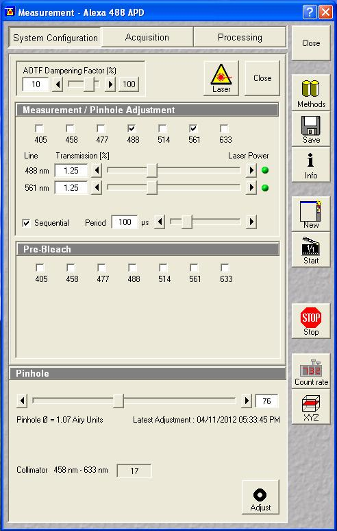
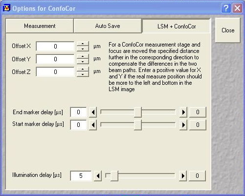
After the add-on is installed, you need to select the appropriate switching settings. I will demonstrate analysis with a switching period of 100 μs with an illumination delay of 5 μs:
Next set up a 1 minute acquisition for the fluorescein solution described above. Set the 488 nm laser power to a reasonable power and set the 561 nm laser power to an arbitrary level (this shouldn't excite the fluorescein anyway). Make sure saving raw data is selected and save the data. The software will save four files: the .fcs file, the two .raw files for each channel and a _Marker.raw file that is supposed to contain the switching offsets but isn't reliable. We will only need the .raw files for this analysis.
Install my ImageJ plugins and open ImageJ. To find the actual switching frequency, run Plugins>Trajectory Tools>calc c3 wlswitch freq jru v1. This plugin basically unmixes the data with a set of switching frequencies (the offsets are independently determined for each) and calculates which one maximizes the ratio between the on and off periods. Select the .raw data set that correspond to the fluorescein emission (typically channel2). I have the plugins set to automatically correct the switching frequency to our default value (9999.889 Hz), so initially enter 10000 for the center frequency. Initially run the plugin with 0.001 Hz resolution (the default). After the plugin completes, there are three outputs: a log output with the frequencies and on/off ratios, a plot of ratio vs. frequency difference from the center values, and a carpet of histograms across the switching period with the vertical axis denoting frequency. Here are example images from our system:
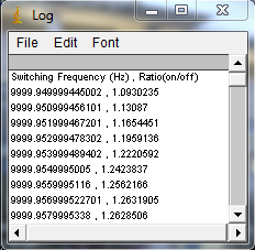
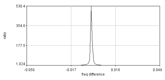
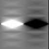
If the program gives a dramatic maximum in the center and a "hole" in the histogram at the center, then rerun the analysis with 0.0001 Hz resolution. The log file will report the optimized frequency at the bottom of the analysis. If you want to plot the histogram across the switching period for reference, use the ImageJ profile plot tool or my Plugins>Image Tools>plot line profile jru v1 tool. If the program does not give a dramatic maximum or the appropriate histogram, you will need to search more broadly for the correct frequency. The log file produces a warning for maximum ratios less than 50 but we routinely obtain ratios of 500. You can do an exhaustive search by increasing the number of searched frequencies (this may take a while) or try decreasing the frequency resolution. Note that decreasing the frequency resolution too much will result in missing the maximum altogether.
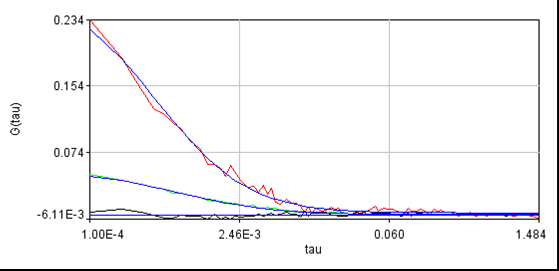
Routine fccs analysis can now be done with the Plugins>Trajectory Tools>analysis cross corr jru v2 plugin. Enter the appropriate sampling frequency from the previous analysis and select Conforcor 3 ALEX in the "File Type?" selection window. There is also an ALEX illumination delay(us) at the bottom which I have defaulted to 2.5. This can be increased to eliminate any remaining bleedthrough at the expense of some collected intensity. The rest of the analysis is performed as described elsewhere on this site. Below is a data set we collected for yeast transformed with EGFP and mCherry constructs which do not interact:
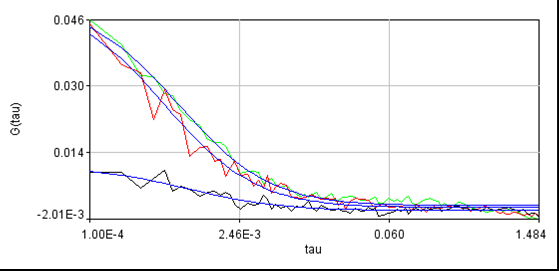
For reference, here is another cell without laser switching:
For those who wish to analyze the data in a program other than the one I have written in ImageJ, I created a new plugin called import c3 wlswitch trajectory jru v1 under Plugins>Trajectory Tools. This also allows for on the fly binning and creation of a histogram across the switching period at the selected frequency. Once you have the trajectory imported, you can export it using the "Save..." button at the bottom of the trajectory window. You can save as a pw file or as a text/binary trajectory with the data type of your choice. Note that these formats require selection of the appropriate data series for export and each channel must be exported separately. Unfortunately, the Zeiss software does not provide import options for file types other than .fcs correlation files or .raw files. Therefore, the Zeiss analysis tools cannot be supported at this time.