Scanning Fluorescence Cross-Correlation (SFCCS) Tutorial.
Scanning FCCS (SFCCS) has become a useful tool at Stowers for determining interactions and dynamics at the yeast nuclear envelope, er, and plasma membrane. This website gives a basic analysis protocol as well as macros for automating this analysis. Please reference our recent JCB paper as well as the previous SFCCS papers below if you publish with this method. The plugins can be downloaded here or as a Fiji update site.
The microscopy requirements for SFCCS are similar to other high sensitivity imaging methods. One needs a highly sensitive confocal with the capability to collect data in line scanning multitrack mode (alternating green and red excitation between lines). We use the Zeiss confocor 3 system with APD detectors but I would anticipate that the Zeiss LSM 780 and a Leica confocal equipped with GaAsP detectors would work as well. Perhaps the most important aspect of the microscope is the ability to collect the redder fluorescent protein signal without exciting the bluer fluorescent protein. In our hands, 514 nm excitation does not excite mTurquoise2 and 561 nm excitation does not excite EGFP. Obviously, the filters also need to be chosen in such a way as to maximize detection efficiency and eliminate collection of the redder fluorescent protein in the blue channel.
The protein requirements for SFCCS are also similar to other high sensitivity imaging methods. Obviously, it is important to test the impact of labeling on protein function. In yeast, the ability to genomically tag allows for fairly straightforward analysis of such effects. In general, we have had the least problems with the GFP family of proteins, while the red proteins have given us more problems. It is also important to note that different fluorescent proteins have differing maturation rates. Given the fast yeast cell cycle time, this can have a fairly dramatic impact. We have had the most success with the mTurqoise2-EYFP pair, though EYFP does struggle with photostability. For that pair, we use 458 and 514 as excitation wavelengths. 440 and 514 should work even better, but those are not available on our systems. We have struggled using 405 nm excitation with mTurquoise2. Another pair we have used with slightly less success is EGFP and mCherry. Here photostability is less of an issue, but mCherry has a tendency to affect protein function. For that pair, we used 488 and 561 as excitation wavelengths.
There are a few more things to consider. For SFCCS measurements, we typically use laser powers on the order of 10 uW at the sample. This is typically measured by choosing a 20x objective with similar transmission to the 40x C Apochromat water objective we use for the actual experiment. We then "image" a power meter somewhat out of focus to get a power measurement. Our pinhole setting for sfccs is typically somewhat bigger than for standard imaging. We routinely use a pinhole setting around 1.5 airy units. Scan speed is obviously set fast enough to be significantly faster than the slowest measured diffusion. For a line size of 512 pixels, our pixel dwell time is typically 6.4 us on the Zeiss system for a line time of 15.3 ms per multitrack line. For the analysis, I typically bin the carpet by 2 in the time dimension for a final time resolution of 30.5 ms. Our pixel size is typically 22 nm. Again for analysis we bin the carpet spatially by 4 and then integrate over a 4 pixel wide region for a total analysis width of ~350 nm (see below).
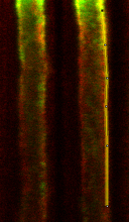
Perhaps the most difficult aspect of sfccs on the nuclear envelope is accounting for motions of the nucleus itself. We typically collect data sets for 5 min. Despite the best yeast immobilization and selection of line, it is inevitable that nuclei will move, drift out of focus, and spindle pole bodies will move into the selected line of interest. While this drift is typically slow compared to the diffusion times of interest, it is strongly correlated between the red and green channels and therefore will result in a strong cross-correlation with a slow diffusion time as seen here. Our approach as well as that of others (Ries and Schwille) has been to track the motion of the membrane and sum the intensity over a region slightly larger than the apparent membrane cross section so that subtle shifts are included in the summed region. It is important to note that this method increases contamination of molecules not bound to the membrane in the signal. For most of our applications this is unimportant given the membrane integral nature of most of our nuclear envelope proteins.
Our method for doing this, then is simply to create a version of the carpet (which was pre-binned 4 x 2) binned in the time dimension by 20. Binning in both cases is accomplished with my Plugins>Stowers>Jay_UnruhImage Tools>bin image jru v1 plugin selecting the cumulative option. A segmented line with a width of 4 pixels (double clicking the line tool in ImageJ brings up the line width tool) is then manually drawn on the carpet, taking care to avoid dramatic bleaching at the start of acquisition and regions which are out of focus or contaminated by spindle pole body intensity. Several examples are shown below.
The Plugins>Stowers>Jay_UnruhCarpet Tools>get line traj jru v1 plugin is then used to pull the drawn region from the pre-binned carpet. Note that different channels should be present in a multi-channel stack prior to running the get line traj jru v1 plugin. If this is not the case, combine the carpets together with Image>Color>merge channels. Final analysis is performed with the Plugins>Stowers>Jay_UnruhTrajectory Tools>analysis cross corr v2 plugin. This analysis is essentially identical to that described here. I typically use a segmented detrending with 3 segments. You can use more or less depending on the diffusion rate of your particular proteins (detrending segments must be much longer than a typical diffusion time) and the severity of bleaching you observe.
I have written a custom macro to semi-automate this process which you can download here. Drag it into ImageJ and select Run Macro from the Macro menu in the window which opens. Note that lines beginning with a "//" are comment lines which are not executed. Some are for notification and others are optional or alternative steps in the analysis. For example, there are options for automated or manual fitting of the correlation curves. Currently the manual version is commented out. If you would like to opt for manual fitting, you should put "//" in front of the automated command and remove it from the manual command. The macro also has commands which ask to save the intermediate plots (the intensity trajectories and the fitted correlation curves). These plots can be opened with Trajectory Tools>import plot jru v1 or by dragging and dropping in FIJI. These lines in the macro can be commented if such steps are not desired.
You can download example wt data sets here for Ndc1-mTurqouise2 vs. Mps3-YFP. It is important to note that the variation between data sets is large and many must be averaged to get a reproducable result. To combine data sets, load all of the desired PlotWindow files into ImageJ and use Plugins>Stowers>Jay_UnruhTrajectory Tools>combine all trajectories jru v1 with the desired data series. Then use Plugins>Stowers>Jay_UnruhTrajectory Tools>average trajectories jru v1 to get the average. You can also get the standard errors. To copy the errors to a spreadsheet program use Plugins>Stowers>Jay_UnruhTrajectory Tools>copy errors jru v1.
Now that you have the numbers, here are some quick calculations you can do. Obviously, the total number of green or red particles is given by γ/G(0)g or γ/G(0)r. The γ factor is defined here. Theoretically for membrane scanning FCCS with a gaussian shaped focal volume, the γ factor should be 0.5 because membrane diffusion is two dimensional. The fraction bound green particles is given by G(0)cc/G(0)r. Likewise the fraction bound red particles is given by G(0)cc/G(0)g.
References:
Chen, J.; Smoyer, C.J.; Slaughter, B.D.; Unruh, J.R.; Jaspersen, S.L. The SUN protein Mps3 controls Ndc1 distribution and function on the nuclear membrane. J. Cell Biol. 2014. 204, 523.
Ries, J. & Schwille, P. Studying slow membrane dynamics with continuous wave scanning fluorescence correlation spectroscopy. Biophys. J. 2006. 91, 1915.
Here are some example images from the attached data set.
Line selection:
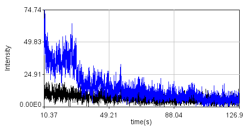
Line profile:
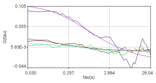
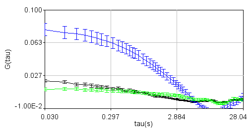
Correlation functions (black-ndc1, blue-nup49, green-cc, red-ndc1fit, magenta-nup49fit, cyan-ccfit):
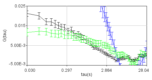
Average correlation functions:
Zoomed to show cross-correlation: